Computing is an essential part of scientific research. Mathematical, engineering, scientific and other technical problems are complex and require computing power and speed. Python provides the SciPy library for solving technical problems computationally.
This article presents a SciPy tutorial and how to implement the code in Python with examples.
Prerequisites
- Installed Python 2.7 or Python 3
- A Python environment for running the code.
- SciPy library installed.
- NumPy library installed (Follow our guide: How to Install NumPy).
- Matplotlib library installed for plotting (optional).
Note: Python 2 no longer has support as of 2020. Consider switching to Python 3. Install Python 3 by following one of our guides: How to install Python 3 on CentOS 7, How to install Python 3 on CentOS 8, How to install Python 3 on Ubuntu, How to install Python on Windows.
What is SciPy?
SciPy (Scientific Python) is an open-source scientific computing module for Python. Based on NumPy, SciPy includes tools to solve scientific problems. Scientists created this library to address their growing needs for solving complex issues.
SciPy vs NumPy
The NumPy library (Numerical Python) does numerical computation. Scientists use this library for working with arrays since NumPy covers elementary uses in data science, statistics, and mathematics.
SciPy covers advanced calculations and functions. This library adds more data science features, all linear algebra functions, and standard scientific algorithms.
Note: Anaconda includes the SciPy, NumPy, and Matplotlib libraries by default. Check out our guides on installing Anaconda: How to Install Anaconda on CentOS 7, How to Install Anaconda on CentOS 8, How to Install Anaconda on Ubuntu.
Why Use SciPy?
The SciPy library builds on top of NumPy and operates on arrays. The computational power is fast because NumPy uses C for evaluation.
The Python scientific stack is similar to MATLAB, Octave, Scilab, and Fortran. The main difference is Python is easy to learn and write.
Note: Some Python environments are scientific. If you need to choose one, check out our comparison of the Best Python IDEs and Code Editors.
SciPy Subpackages
The SciPy library has different groups of subpackages. There are two ways to import subpackages from the SciPy module:
import scipy.<sub package name> as <alias>Or alternatively:
from scipy import <sub package name> as <alias>In both importing methods, the alias is optional.
SciPy Functions
SciPy includes many of the primary array functions available in NumPy and some of the commonly used modules from the SciPy subpackages.
To import a function from a subpackage, use:
from scipy.<subpackage> import <function>Note: Some of the NumPy functions available in SciPy show deprecation warnings.
Basic Functions
To get help and information for any SciPy function, use the help() command:
help(<name of function>)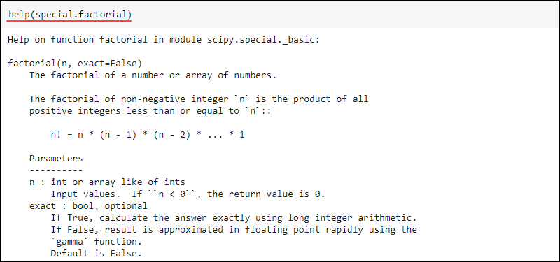
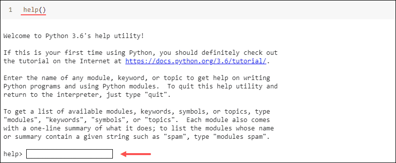
The help() command does not need parameters. After executing without parameters, a prompt appears where you input the function name.
Another quick way to get help with any command in Python is to write the command name, put a question mark at the end, and run the code.
Special Functions
Special functions in the SciPy module include commonly used computations and algorithms. All special functions accept NumPy arrays as input. The calculations are elementwise.
To import the special subpackage, use:
import scipy.special as specialOr alternatively:
from scipy import specialTo import a specific function from the special subpackage, use:
from scipy.special import <function name>Factorial
Evaluate the factorial of any number by running:
special.factorial(<integer or array>)For example, to find the factorial of ten, use:
special.factorial(10)
Permutations and Combinations
To find the number of permutations, use:
special.perm(<number of elements>, <number of elements taken>)For example, to see the number of permutations of three elements taken two at a time:
special.perm(6,2)
Similarly, find the number of combinations with:
special.comb(<number of elements>, <number of elements taken>, repetition=<True or False>)To find the number of combinations of three elements taken two at a time with repetition, enter:
special.comb(6,2, repetition=True)
Permutations and combinations are used in computer science sorting algorithms.
Exponential Functions
Exponential functions evaluate the exponents for different bases.
Calculate the exponents of base ten with:
special.exp10(<integer or array>)For example:
special.exp10([0,1,2])
Computer science often uses exponential functions of base two:
special.exp2(<integer or array>)Calculate the tenth power of base two with:
special.exp2(10)
Logarithmic Sum of Exponentials
The Logarithmic Sum of Exponentials (LSE or LogSumExp) is an approximation used by machine learning algorithms. Calculate the LSE with:
special.logsumexp(<integer or array>)
Bessel Function
Bessel functions appear in wave propagation, signal processing, and static potential problems. Find the Bessel function of the first kind with:
special.jn(<integer order>, <integer or array>)Take advantage of the full stack to visualize the Bessel function. To find the second-order Bessel function of the first kind, use:
#import stack
import scipy.special as special
import matplotlib.pyplot as plt
import numpy as np
#The X-axis
x = np.linspace(1,50,100)
#Bessel function of the first kind order two
jn1 = special.jn(2,x)
Plot the results:
#Plotting
plt.title('Bessel function first kind order two')
plt.plot(x, jn1)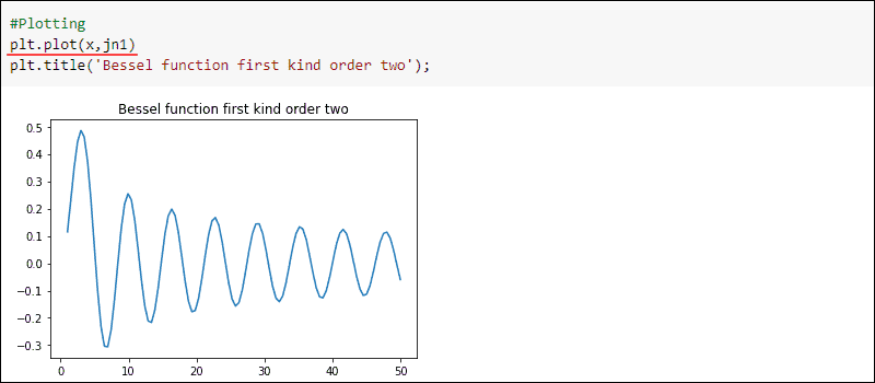
Note: Learn about a crucial mathematical operation in Python, raising a number to a power by reading our article Python Power Operator and Function.
Integration and ODE Functions
SciPy provides a subpackage for calculations with definite integrals. To import the integrate subpackage, use:
import scipy.integrate as integrateOr alternatively:
from scipy import integrateImport a specific function from the subpackage integrate with:
from scipy.integrate import <function name>General Integration
Calculate a single variable integral with the quad function from the integrate subpackage:
integrate.quad(<function>, <lower limit>, <upper limit>)The function input is defined using a lambda function.
For example, to calculate the definite integral of the function x+1 between zero and one:
from scipy import integrate
f = lambda x: x+1
integrate.quad(f, 0, 1)
The output shows two values. The first value is the evaluated integral, and the second is the error of estimation.

Optimization Functions
SciPy has an optimization subpackage for finding the minimum or maximum of a function. The optimize subpackage includes solvers and algorithms for finding local and global optimal values.
To import the optimize subpackage:
from scipy import optimizeOr use:
import scipy.optimize as optimizeTo import a specific function from the subpackage optimize, run:
from scipy.optimize import <function name>Minimize a Function
Finding a minimum of a function is used in machine learning to lower an algorithm’s loss (or error).
For example, you can create a function and find the minimum. To do so, use the fmin function from the optimize subpackage in SciPy:
#Import stack
import numpy as np
from scipy import optimize
#Defining inverse sine function
def f(x):
    return -np.sin(x)
#X-axis
x = np.linspace(0,5,100)
#Starting point
start = 3
#Simplex algorithm for optimization
optimized = optimize.fmin(f,start)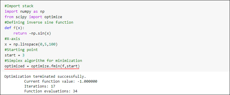
To plot the result, run:
import matplotlib.pyplot as plt
plt.plot(x, f(x))
plt.scatter(start,f(start))
plt.scatter(optimized, f(optimized))
plt.legend(['Function -sin(x)', 'Starting point', 'Optimized minimum'])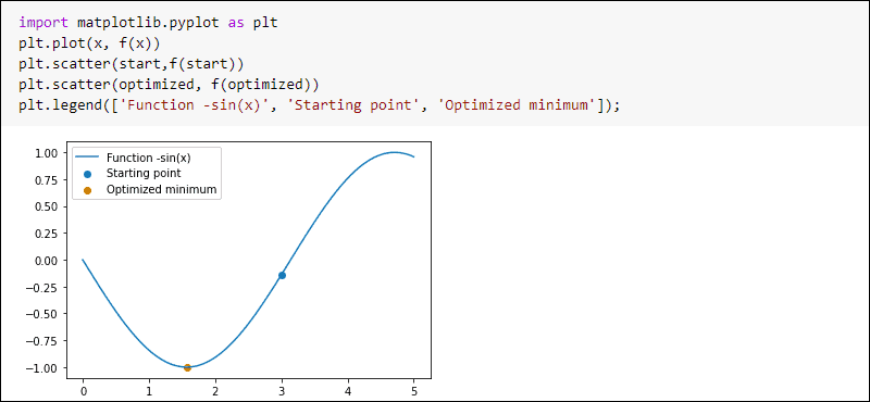
Fourier Transformation Functions
SciPy includes a subpackage for Fourier transformation functions called fftpack. The transformations are Discrete Fourier Transformations (DFT). All transforms are applied using the Fast Fourier Transformation (FFT) algorithm.
To import the fftpack subpackage, use:
import scipy.fftpack as fftpackOr:
from scipy import fftpackFast Fourier Transform
As an example, create a periodic function as a sum of three sine waves:
import numpy as np
freq_samp = 100
#Time
t = np.linspace(0, 1, freq_samp*2, endpoint = False )
#Frequencies
f1, f2, f3 = 1, 5, 20
#Amplitudes
A1, A2, A3 = 3, 2, 1
x1 = A1*np.sin(f1*2*np.pi*t)
x2 = A2*np.sin(f2*2*np.pi*t)
x3 = A3*np.sin(f3*2*np.pi*t)
#Sum of waves
x = x1+x2+x3
Plot the waves using matplotlib:
import matplotlib.pyplot as plt
plt.subplot(2,1,1)
plt.plot(t,x1,t,x2,t,x3)
plt.subplot(2,1,2)
plt.plot(t,x)
plt.xlabel('Time (s)')
plt.ylabel('Amplitude');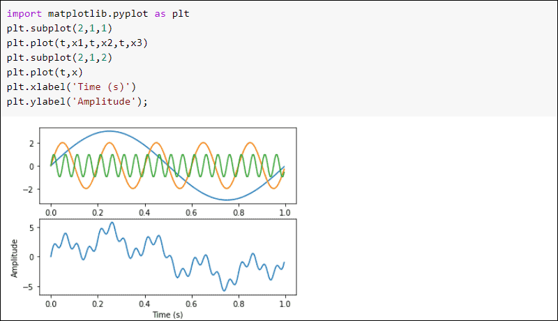
Next, apply the fft and fftfreq functions from the fftpack to do a Fourier transform of the signal.
from scipy import fftpack
A = fftpack.fft(x)
freq = fftpack.fftfreq(len(x))*freq_samp*2
Plot the results to see the frequency domain:
plt.stem(freq,np.abs(A)/freq_samp,use_line_collection=True)
plt.xlim(-25,25)
plt.xlabel('Frequency (Hz)')
plt.ylabel('Amplitude')
plt.grid()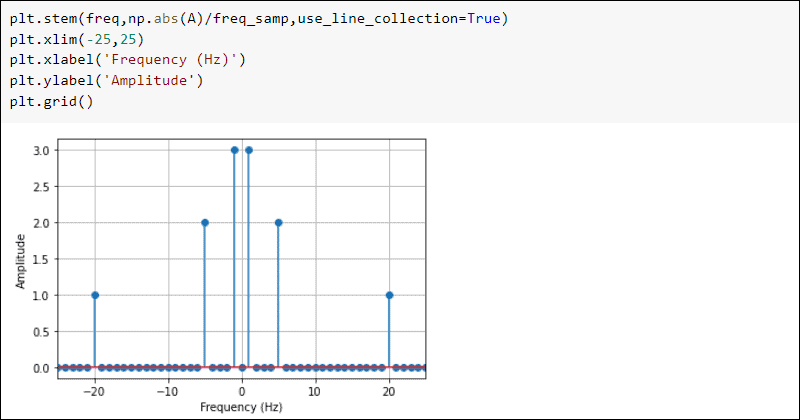
Signal Processing Functions
The subpackage signal includes functions used in signal processing. To import signal, run:
import scipy.signal as signalOr alternatively:
from scipy import signalConvolution
A common task in signal processing is convolution. The SciPy subpackage signal has the function convolve to perform this task. For example, create two signals with different frequencies:
import numpy as np
#Time
t = np.linspace(0,1,100)
#Frequency
f1, f2 = 5, 2
#Two signals of different frequencies
first_signal = np.sin(f1*2*np.pi*t)
second_signal = np.sin(f2*2*np.pi*t)
Plot the signals:
import matplotlib.pyplot as plt
#Plotting both signals
plt.subplot(2,1,1)
plt.plot(t, first_signal)
plt.subplot(2,1,2)
plt.plot(t, second_signal)
plt.ylabel('Amplitude')
plt.xlabel('Time (s)')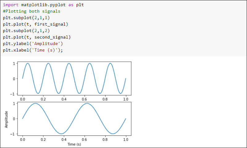
Import the signal subpackage from scipy. Use the convolve function from the signal subpackage to convolve the two signals:
#Importing the signal subpackage
from scipy import signal
#Convolving two signals
convolution = signal.convolve(first_signal, second_signal, mode='same')
Plot the results:
#Plotting the result
plt.plot(t, convolution)
plt.xlabel('Time (s)')
plt.ylabel('Amplitude')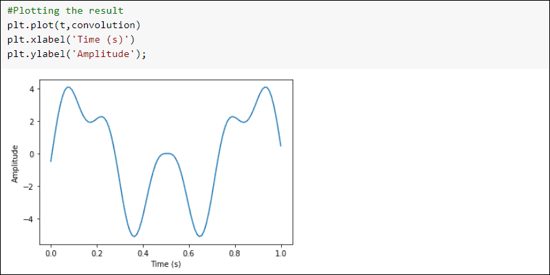
Interpolation Functions
Interpolation is used in the numerical analysis field to generalize values between two points. SciPy has the interpolate subpackage with interpolation functions and algorithms.
Import the interpolate subpackage with:
import scipy.interpolate as interpolateOr:
from scipy import interpolateOne Dimensional Interpolation
The SciPy interpolate subpackage has the interp1d function for one dimensional interpolation of data. As an example, create toy data using numpy:
import numpy as np
#Create toy data
x = np.arange(0,10,0.5)
y = np.sin(x)
Interpolate the data with interp1d from the interpolate subpackage:
from scipy import interpolate
#Interpolate
f = interpolate.interp1d(x, y)
#Create interpolation function
x_i = np.arange(0,10,3)
y_i = f(x_i)
Plot the results:
#Plot results
plt.scatter(x,y)
plt.plot(x_i, y_i)
plt.legend(['Interpolation', 'Data points'])
Linear Algebra
SciPy has a fully-featured linear algebra subpackage. The SciPy linear algebra subpackage is optimized with the ATLAS LAPACK and BLAS libraries for faster computation.
To import the linear algebra package from SciPy, run:
import scipy.linalg as linalgOr use:
from scipy import linalgAll the linear algebra functions expect a NumPy array for input.
Determinant
Calculate the determinant of a matrix with det from the linalg subpackage:
linalg.det(<numpy array>)For example:
import numpy as np
#Generate a 2D array
A = np.array([[1,2],[3, 4]])
from scipy import linalg
#Calculate the determinant
linalg.det(A)
Inverse Matrix
Determine the inverse matrix by using inv:
linalg.inv(<numpy array>)For example:
import numpy as np
#Generate a 2D array
A = np.array([[1,2],[3,4]])
from scipy import linalg
#Calculate the inverse matrix
linalg.inv(A)
Eigenvectors and Eigenvalues
Eigenvectors and eigenvalues are a matrix decomposition method. The eigenvalue-eigenvector problem is a commonly implemented linear algebra problem.
The eig function finds the eigenvalues and eigenvectors of a matrix:
linalg.eig(<numpy array>)The output returns two arrays. The first contains eigenvalues, and the second has eigenvectors for the given matrix. For example:
import numpy as np
#Generate a 2D array
A = np.array([[1,2],[3, 4]])
from scipy import linalg
#Calculate the eigenvalues and eigenvectors
linalg.eig(A)
Spatial Data Structures and Algorithms
Spatial data structures are objects made of points, lines, and surfaces. SciPy has algorithms for spatial data structures since they apply to many scientific disciplines.
Import the spatial subpackage from SciPy with:
import scipy.spatial as spatialOr:
from scipy import spatialA notable example of a spatial algorithm is the Voronoi diagram. For a given set of points, Voronoi maps divide a plane into regions. If a new point falls into a region, the point in the region is the nearest neighbor.
Note: Voronoi diagrams relate to the k-Nearest Neighbor algorithm in machine learning.
As an example, create a Voronoi diagram from twenty random points:
from scipy.spatial import Voronoi
import numpy as np
points = np.random.rand(20,2)
voronoi = Voronoi(points)
from scipy.spatial import voronoi_plot_2d
fig = voronoi_plot_2d(voronoi,show_vertices=False)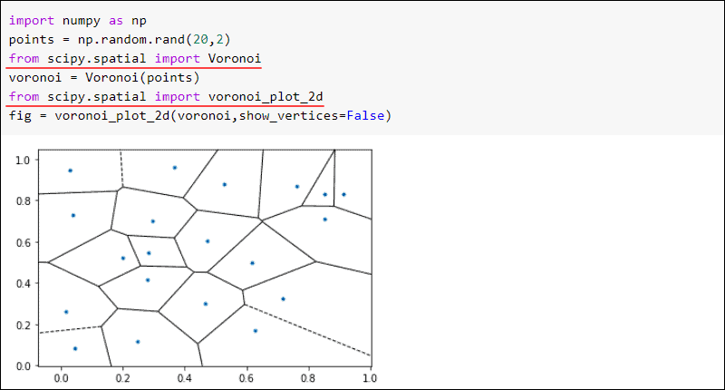
Image Processing
SciPy has a subpackage for various n-dimensional image processing. To import the ndimage subpackage, run:
import scipy.ndimage as ndimageOr use:
from scipy import ndimageThe SciPy misc subpackage contains a sample image for demonstration purposes. To import the misc subpackage and show the image:
from scipy import misc
from matplotlib import pyplot as plt
raccoon = misc.face()
#show image
plt.imshow(raccoon)
plt.show()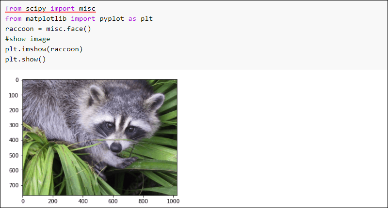
Import the ndimage subpackage and apply a uniform_filter to the image. Show the image to see the results:
from scipy import ndimage
filtered = ndimage.uniform_filter(raccoon)
plt.imshow(filtered)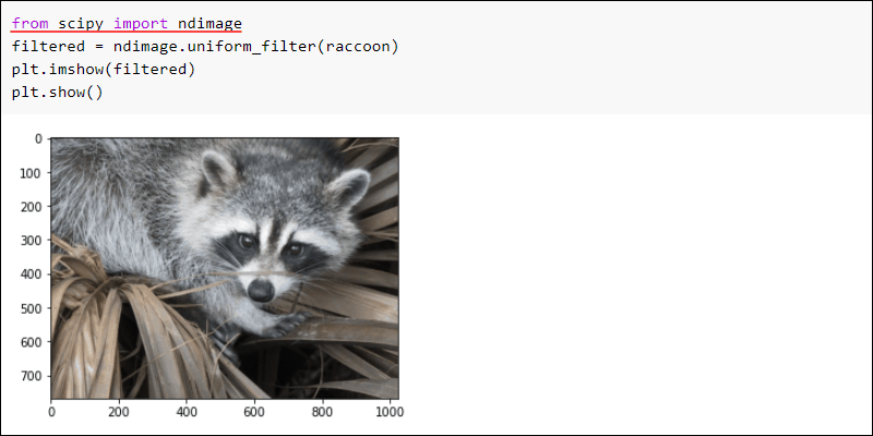
File IO (File Input / Output Package)
SciPy has a file input and output subpackage called io. The io subpackage is used for reading and writing data formats from different scientific computing programs and languages, such as Fortran, MATLAB, IDL, etc.
Import the io subpackage from SciPy with:
import scipy.io as sioOr use:
from scipy import io as sioConclusion
This tutorial provided the necessary ScyPy examples to get started. Python is easy to learn for beginners and scripts are simple to write and test. Combining SciPy with other Python libraries, such as NumPy and Matplotlib, Python becomes a powerful scientific tool. The SciPy subpackages are well documented and developed continuously.
For further reading, check out our tutorial on the Pandas library: Introduction to Python Pandas.


