How to Find Standard Deviation in R

Standard deviation is one of the most fundamental measures of variability in statistics. In R, there are multiple ways to compute the standard deviation: from simple, built-in functions to grouped and weighted calculations.

This tutorial will explain the standard deviation concept and present practical examples for each scenario.

Prerequisites

• R installed (install R on Ubuntu).
• Access to the terminal.

What Is Standard Deviation?

Standard deviation measures how far individual observations deviate from the average of the dataset. A low standard deviation means the values cluster closely around the mean. A high standard deviation indicates that the data is widely spread.

Mathematically, standard deviation is the square root of variance. For a dataset x1,x2,...,xnx_1, x_2, ..., x_nx1​,x2​,...,xn​, the sample standard deviation is calculated as:

s = √( Σ (xi – x̄)² / (n − 1) )

Where:

• x̄ is the sample mean.
• n is the number of observations.
• Σ represents summation.

The denominator uses n − 1 instead of n. This adjustment, called Bessel's correction, ensures an unbiased estimate when working with samples instead of full populations.

Because the result is expressed in the same unit as the original data, standard deviation is easier to interpret than variance.

Standard Deviation in Data Analysis

In data analysis, standard deviation is important because it provides context for averages. A mean alone tells you the center of a dataset, but it does not reveal how reliable or stable that value is. Standard deviation shows whether observations are tightly clustered or widely scattered, which directly affects how trends and decisions are interpreted.

Standard deviation is heavily used in finance, quality control, scientific research, machine learning, and performance analytics. Analysts rely on it to measure volatility, detect anomalies, evaluate experimental consistency, and assess risk. In predictive modeling, it helps normalize features and compare variables that operate on different scales.

In practice, analysts use standard deviation to:

• Compare variability between datasets.
• Identify outliers or unusual behavior.
• Build confidence intervals.
• Standardize variables (z-scores).
• Evaluate data consistency.

Standard deviation should not be interpreted in isolation. Since it is sensitive to outliers, pairing it with metrics such as the median or the interquartile range provides a more complete view of the distribution.

How to Find Standard Deviation in R

R includes built-in statistical tools, but understanding how the calculation works internally helps avoid mistakes. The sections below show both a manual implementation and the standard function most users rely on.

Find Standard Deviation via Naive Approach

The naive approach calculates standard deviation by directly implementing the mathematical formula. Instead of relying on R's built-in helpers, the user manually computes the mean, the squared deviations, and the final square root.

This method is mainly educational. It helps understand what standard deviation actually measures and how statistical software arrives at the result. It is also useful when you need full control over the formula in custom statistical workflows.

You can run the following example in the R console, RStudio, or inside an R script file. The code walks through each step of the formula explicitly:

x <- c(12, 24, 74, 32, 14, 29, 84, 56)

manual_sd <- sqrt(sum((x - mean(x))^2) / (length(x) - 1))
manual_sd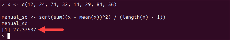

The expression subtracts the mean from each value, squares the differences, averages them using n − 1, and takes the square root. The result matches what R's built-in function produces.

Although this approach is rarely used in production analysis, it builds intuition and helps validate statistical computations.

Find Standard Deviation via sd()

In practical data analysis, we recommend using R's built-in sd() function. It performs the same calculation as the manual approach but is faster, safer, and easier to read. This is the standard method used in real projects.

The function expects a numeric vector and returns the sample standard deviation. Run the following in your R console or script:

data <- c(5, 10, 15, 20, 25)
sd(data)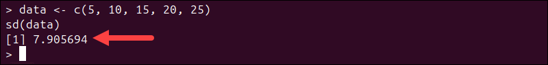

Real datasets often contain missing values. By default, sd() returns NA if any value is missing, which can silently break analysis pipelines.

To ignore missing entries, add the na.rm argument:

sd(data, na.rm = TRUE)

This argument tells R to remove missing values before computing the result. In practice, you should always consider whether missing data should be removed, imputed, or investigated before continuing analysis.

Other Standard Deviation Operations in R

The basic sd() function works for simple vectors, but real-world datasets are rarely completely clean. Analysts often need to compute the standard deviation for entire populations, grouped categories, multiple columns, or weighted observations.

The sections below explain how each scenario differs conceptually and how to run the calculations in practice.

Find Population Standard Deviation in R

The standard deviation returned by sd() is a sample standard deviation, which assumes your data represents a subset of a larger population. When you are working with the entire population, the formula changes slightly.

Population standard deviation divides by n instead of n − 1. This formula removes Bessel's correction because it no longer estimates variability but measures it directly. Use this approach when your dataset contains every possible observation, such as full census data or complete system logs.

Run the following code in your R console or script:

x <- c(12, 24, 74, 32, 14, 29, 84, 56)

pop_sd <- sqrt(mean((x - mean(x))^2))
pop_sd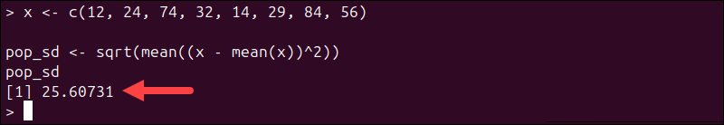

This formula calculates the population standard deviation manually using the correct denominator.

Find Grouped Standard Deviation in R

Grouped standard deviation measures variability within categories instead of across the entire dataset. This is useful when analyzing departments, regions, user segments, or experimental groups.

Instead of one global value, you get a standard deviation for each group, allowing comparisons between categories. The results reveal which groups are more consistent or volatile.

R provides several tools for grouped calculations. The best choice depends on whether you prefer base R or tidyverse workflows.

via tapply()

tapply() is a base R function that splits a vector into subsets and applies a function to each subset. It is lightweight and ideal for quick, grouped summaries.

The arguments are:

• The numeric values,
• The grouping variable,
• Function to apply (sd in this case).

Run the following in your console or script:

values <- c(10, 12, 13, 15, 20, 22)
groups <- c("A", "A", "B", "B", "A", "B")

tapply(values, groups, sd)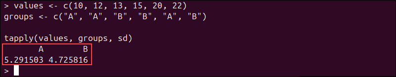

R automatically separates the data into groups A and B and returns the standard deviation for each group.

via aggregate()

aggregate() works with data frames and produces structured output. It is useful when your data already lives in tabular format, and you want results that stay organized.

The syntax uses the following formula:

numeric_column ~ group_column

Execute the following:

df <- data.frame(
  group = c("A","A","B","B"),
  score = c(5,8,7,9)
)

aggregate(score ~ group, data = df, sd)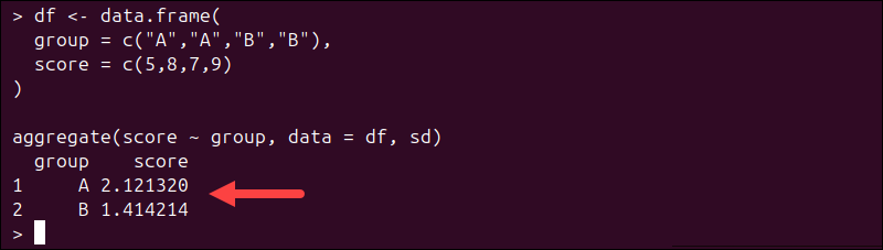

The result is a new data frame containing grouped standard deviations.

via dplyr

The dplyr package provides a modern pipeline-based workflow. It is preferred in larger analysis projects because it reads like a sequence of instructions.

install.packages("dplyr")

First load the package, then group and summarize:

library(dplyr)

df %>%
  group_by(group) %>%
  summarise(sd_score = sd(score))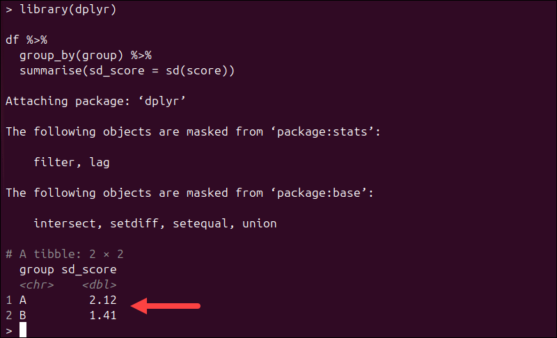

This approach integrates smoothly with data cleaning and transformation pipelines.

Find Column-Wise Standard Deviation

Column-wise standard deviation calculates variability for each numeric column in a data frame. This is common in exploratory analysis and feature engineering.

Instead of writing sd() for each column manually, you can apply it across all columns at once.

Run the following:

df <- data.frame(a = rnorm(10), b = rnorm(10))

sapply(df, sd)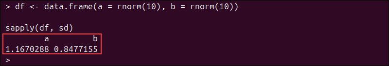

The output is a named vector containing the standard deviation for each column. For very large datasets, performance-focused packages such as matrixStats offer faster implementations.

Find Weighted Standard Deviation

Weighted standard deviation accounts for observations that contribute unequally. This is important in survey analysis, scoring systems, and aggregated datasets where some values represent larger populations.

R does not include a built-in weighted SD function, so it needs to be computed manually:

1. Calculate the weighted mean.

2. Compute weighted squared deviations.

3. Take the square root.

Run the following:

values <- c(2, 4, 6)
weights <- c(1, 2, 1)

w_mean <- sum(values * weights) / sum(weights)
w_sd <- sqrt(sum(weights * (values - w_mean)^2) / sum(weights))
w_sd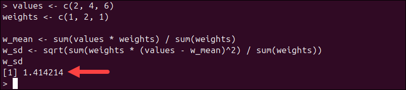

This produces a weighted standard deviation consistent with statistical definitions.

Mistakes When Working with Standard Deviation in R

Even though standard deviation is a simple concept, small implementation mistakes can produce incorrect or misleading results. Most issues stem from data types, missing values, or misunderstandings of what sd() computes.

The sections below describe common problems, why they happen, and how to fix them in practice.

Using sd() on Non-Numeric Data

The sd() function only works on numeric vectors. If your data contains characters, factors, or lists, R cannot compute deviations and throws an error.

This usually happens when importing CSV files or working with mixed-type data frames, where numeric columns may be accidentally stored as text.

If you see an error like:

Error in sd(x) : 'x' must be numeric

That means you must convert the data before running the calculation. Run the following:

x <- c("1", "2", "3")

sd(as.numeric(x))

Or select the numeric column explicitly from a data frame with:

sd(df$numeric_column)

Always verify data types using str(df) before running statistical functions.

Forgetting na.rm = TRUE

Missing values (NA) propagate through statistical calculations. If even a single missing value is present, sd() returns NA by default. This behavior prevents silent data loss, but it often surprises beginners.

For example:

x <- c(5, 10, NA, 20)
sd(x)

The code returns NA:

To ignore missing values and continue the calculation, run:

sd(x, na.rm = TRUE)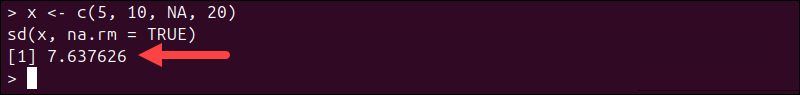

You should only remove missing values when it makes sense analytically. In some cases, missing data may signal a deeper data quality issue that needs investigation.

Confusing Sample vs. Population Standard Deviation

A common misconception is that sd() calculates the population standard deviation. However, it computes the sample standard deviation using n − 1. This matters in scientific, financial, and modeling workflows where the distinction changes interpretation.

For population standard deviation, compute manually by using:

pop_sd <- sqrt(mean((x - mean(x))^2))
pop_sd

Use sample SD when working with subsets or estimates. Use population SD only when your dataset contains the full population.

Conclusion

This tutorial explained how to use R to calculate the standard deviation. To compute standard deviation in R, use built-in functions, manual formulas, or grouped and weighted approaches depending on your dataset and analysis needs.

Next, learn about the differences between R and Python.